Model Information
Introduction
CE-QUAL-W2 is a two-dimensional water quality and hydrodynamic code supported by the USACE Waterways Experiments Station (Cole and Buchak [1]). The model has been widely applied to stratified surface water systems such as lakes, reservoirs, and estuaries and computes water levels, horizontal and vertical velocities, temperature, and 21 other water quality parameters (such as dissolved oxygen, nutrients, organic matter, algae, pH, the carbonate cycle, bacteria, and dissolved and suspended solids). A typical model grid is shown in Figure 1 where the vertical axis is aligned with gravity.
This paper documents the development of CE-QUAL-W2 Version 3 incorporating sloping riverine sections. Version 3 has the capability of modeling entire river basins with rivers and inter-connected lakes, reservoirs, and/or estuaries. Four example applications are shown illustrating the use of Version 3.
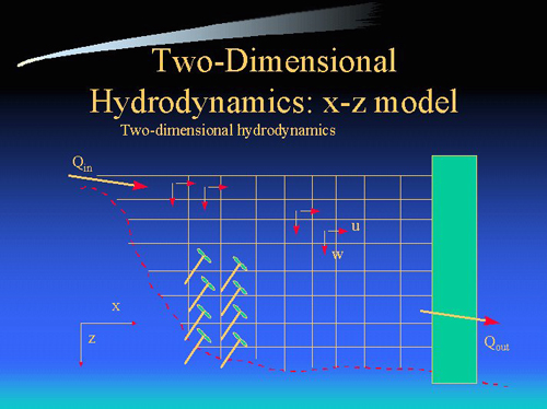
Figure 1. Typical CE-QUAL-W2 Version 2 model grid.
Development Rationale
CE-QUAL-W2 has been in use for the last two decades as a tool for water quality managers to assess the impacts of management strategies on reservoir, lake, and estuarine systems. A predominant feature of the model is its ability to compute the two-dimensional velocity field for narrow systems that stratify. In contrast with many reservoir models that are zero-dimensional with regards to hydrodynamics, the ability to accurately simulate transport can be as important as the water column kinetics in accurately simulating water quality.
A limitation of Version 2 is its inability to model sloping riverine waterbodies. Models, such as WQRSS (Smith [2]), HEC-5Q (Corps of Engineers [3]), and HSPF (Donigian,et al. [4]), have been developed for river basin modeling but have serious limitations. One issue is that the HEC-5Q (similar to WQRSS) and HSPF models incorporate a one-dimensional, longitudinal river model with a one-dimensional, vertical reservoir model (one-dimensional for temperature and water quality and zero dimensional for hydrodynamics). The modeler must choose the location of the transition from 1-D longitudinal to 1-D vertical. Besides the limitation of not solving for the velocity field in the stratified, reservoir system, any point source inputs to the reservoir section are spread over the entire longitudinal distribution of the reservoir layer.
Other hydraulic and water quality models in common use for unsteady flow include the 1-D dynamic EPA model DYNHYD (Ambrose,et al. [5]), used together with the multidimensional water quality model WASP. WASP relies on DYNHYD for 1-D hydrodynamic predictions. If WASP is used in a multi-dimensional schematization, the modeler must specify dispersion coefficients to allow transport in the vertical and/or lateral directions or use another hydrodynamic model that explicitly includes these effects. Also, the Corps model, CE-QUAL-RIV1 (Environmental Laboratory [6]), is a one-dimensional dynamic flow and water quality model used for one-dimensional river or stream sections. None of these models have the ability to characterize adequately the hydraulics or water quality of deeper reservoir systems or deep river pools that stratify.
In the original development of CE-QUAL-W2, vertical accelerations were considered negligible compared to gravity forces. This assumption lead to the hydrostatic pressure approximation for the z-momentum equation. In sloping channels, this assumption is not always valid because vertical accelerations cannot be neglected if the z-axis is aligned with gravity. Also, the current Version 2 algorithm does not allow the upstream bed elevation to be above the downstream water surface elevation. Because watershed and river basin modeling is becoming more important for water quality managers, providing the capability for CE-QUAL-W2 to be used as a complete tool for river basin modeling is an essential step in improving the current state-of-the-art.
Development Approach
There were many approaches that could have been implemented to incorporate riverine branches within CE-QUAL-W2. By choosing a theoretical basis for the riverine branches that uses the existing CE-QUAL-W2 2-D computational scheme for hydraulics and water quality, the following benefits accrued:
-
Code updates in the computational scheme affected the entire model rather than just one of the computational schemes for either the riverine or the reservoir sections leading to easier code maintenance.
-
No changes were made to the temperature or water quality solution algorithms.
-
By using the two-dimensional framework, the riverine branches had the ability to predict the velocity and water quality field in two dimensions - this has advantages in modeling the following processes: sediment deposition and scour, particulate (algae, detritus, suspended solids) sedimentation, and sediment flux processes as well as making Manning’s friction factor stage invariant.
-
Since the entire watershed model had the same theoretical basis, setting up branches and interfacing branches involved the same process whether for reservoir or riverine sections, thus making code maintenance and model set-up easier.
The theoretical approach was to re-derive the governing equations assuming that the 2-D grid is adjusted by the channel slope (Figure 2).
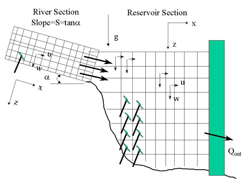
Figure 2. Conceptual schematic of river-reservoir connection.
Theoretical Basis
Details of deriving the governing equations for CE-QUAL-W2 Version 3 for the river basin model are given in Wells [8]. Table 1 shows the governing equations after lateral averaging for a channel slope of zero (original model formulation) and for an arbitrary channel slope.
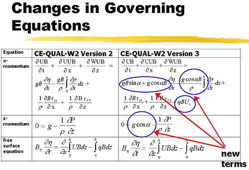
Table 1. Comparison of governing equations for CE-QUAL-W2 with and without channel slope.
Note: U,W: horizontal and vertical velocity, B: channel width, P: pressure, g: acceleration due to gravity,tx,tz: lateral average shear stress in x and z,r: density,h: water surface,a: channel angle, Ux: x-component of velocity from side branch, q: lateral inflow per unit length
Numerous algorithmic changes were made in the CE-QUAL-W2 model. In addition to the general channel sloping feature, these changes include the ability to choose:
-
Turbulence closure models for each waterbody using eddy-viscosity mixing length models.
-
Varying vertical grids between waterbodies.
-
Chezy or Manning's friction factor.
-
Reaeration formulae based on the riverine or reservoir/lake or estuary character of the waterbody or user-defined formulations.
-
Evaporation models based on theory or user-defined formulations.
-
The ability to linearly link one branch with another or specify an internal dam or internal hydraulic structure(s) (spillways, gates, weirs, and pipes) within or between water bodies (The pipes algorithm is an unsteady 1-D hydrodynamic sub-model to the core W2 code from Berger and Wells [9].
-
The effect of hydraulic structures on gas transfer and total dissolved gas transport.
-
Conservation of longitudinal momentum at intersections between main branches and side branches.
-
The effect of lateral inflows from tributaries or the lateral component of inflows from branch. intersections on the vertical eddy viscosity
-
QUICKEST/ULTIMATE numerical transport scheme.
-
Implicit eddy viscosity formulation that removes its timestep requirement.
-
Multiple user defined algal groups.
-
Multiple user defined organic matter groups.
-
Sediment diagenesis model.
Test Applications
Richard B. Russell (RBR)/J. Strom Thurmond (JST)
RBR and JST (previously known as Clarks Hill Lake as shown in figure 3) are Corps Reservoirs located on the Savannah River between Georgia and South Carolina. JST is located immediately below RBR. The study involved investigating the effects of proposed pump-storage operations on temperature and water quality for the two reservoirs. This required a rewrite of the code in order to dynamically link the two systems. The linkage algorithm was sufficiently generalized to allow dynamic linkage to any number of "waterbodies". During algorithm development, it was recognized that a natural extension would be to allow modeling of the river reaches in between reservoirs thus providing a state-of-the-art waterbasin management tool that would handle reservoir hydrodynamics, temperatures, and water quality in a realistic manner.
Figure 3. Map of Richard B. Russell and J. Strom Thurmond (Clarks Hill) Reservoirs.
Prior to 1996, both reservoirs were operated for peaking hydropower. During the course of the study, extensive pump-storage operations were conducted in 1996 and data were collected that allowed evaluation of the model's ability to simulate the effects of pump-storage on temperature and DO in the two reservoirs.
All hydrodynamic/temperature calibration parameters including longitudinal eddy viscosity/diffusivity, bottom friction, sediment heat exchange, and short wave solar radiation absorption/extinction were set to their default values with the exception of the wind-sheltering coefficient, which was set to 0.9 for RBR and 1.0 for JST. The wind-sheltering coefficient is used to multiply observed winds in order to decrease the effective wind reaching the reservoir surface.
Temperature simulations
The model was calibrated to data collected during 1988, 1994, and 1996. The year 1988 represents a low flow year, 1994 represents a high flow year, and 1996 represents an average flow year with extensive pump-storage operations.
Figures 1-3 show the results of the model simulations for the calibration years for RBR while Figures 4-6 show the results for JST. The x’s represent observed data and the lines represent model predictions. The x’s are scaled to represent±0.5°C. Additionally, the absolute mean error (AME) and the root mean square error (RMS) are presented on the plots as a further aid in evaluating model predictions.
The results show that the model is capable of reproducing the observed temperatures in both RBR and JST under varying flow years and reservoir operations. Additionally, the model captured the approximate 4°C increase in hypolimnetic temperatures for 1996 compared to 1988 and 1994 due to pump-storage operations.
Figure 4: 1988 RBR computed versus observed temperature.

Figure 5: 1994 RBR computed versus observed temperature.

Figure 6: 1996 RBR computed versus observed temperature.
Figure 7: 1988 JST computed versus observed temperature.
Figure 8: 1994 JST computed versus observed temperature.
Figure 9: 1996 JST computed versus observed temperature.
Dissolved Oxygen Simulations
An additional complication to this study was the presence of an oxygen diffuser system that had to be incorporated into the model in order to reproduce observed DO in RBR. The oxygen diffuser system consists of one system located in the forebay and another located approximately 1.6 km upstream from the dam. During 1988, most oxygen injection occurred in the forebay except during late summer when the upstream system was also used. Oxygen injection during 1994 utilized both of the systems, while in 1996 the upstream system was the only one utilized.
Figures 10-13 show the results of 1988, 1994, and 1996 DO simulations for RBR for the station located closest to the dam. The simulations included the full suite of algal/nutrient/DO interactions available in the model. Sediment oxygen demand (SOD) was modeled using a first-order sediment compartment that included the effects of organic matter delivery to and subsequent decay in the sediments for both allochthonous and autochthonous sources of organic matter. Additionally, a zero-order sediment oxygen demand was included to provide for background SOD.
Observed DO in RBR exhibits very complex patterns in response to the oxygen injection system, algal production, peaking hydropower operations, and, in 1996, pump-storage operations. For 1988 and 1994, the DO regime exhibits a pronounced metalimnetic minimum due to the oxygen injection system delivering oxygen to the hypolimnion. In contrast, the metalimnetic DO minimum is greatly reduced in 1996 due to the effects of pump-storage that caused greater hypolimnetic mixing (Figure 13). Although not normally thought of when calibrating for hydrodynamics, DO in RBR provides a much better indication of how well the model is reproducing reservoir hydrodynamics because of the very dynamic interactions of peaking-hydropower, pump-storage, and oxygen injection operations.

Figure 10. 1988 RBR computed versus observed DO, March-June.
Figure 11: 1988 RBR computed versus observed DO, June-October.

Figure 12. RBR 1994 computed versus observed DO.
Figure 13: 1996 RBR computed versus observed DO.
Figure 14 illustrates the model’s ability to capture the longitudinal gradients in DO along the mainstem as well as the differences in DO between side branches and the mainstem during July of 1996. CE-QUAL-W2 reproduces the anoxic hypolimnion for the two stations located off the mainstem as well as reproducing the differences between the two stations. The model also reproduces the effects of additional hypolimnetic oxygen delivery upstream of the oxygen diffuser system due to pump-storage operations advecting higher DO upstream.

Figure 14: 1996 RBR computed versus observed DO during July. The first two plots are stations located on side branches off the mainstem. The last five plots are stations located at the upstream portion of the mainstem down to the dam.
Figures 15-17 show the results of the 1988, 1994, and 1996 DO simulations for JST. The DO regime in JST is quite different from that in RBR, although JST also exhibits a metalimnetic DO minimum. The model captures much of the DO dynamics in JST. However, the metalimnetic DO minimum is not captured as accurately as in RBR.
Figure 15: 1988 JST computed versus observed DO.
Figure 16: 1994 JST computed versus observed DO.
Figure 17: 1996 JST computed versus observed DO.
Lower Snake River
The domain of the Lower Snake River from C. J. Strike Reservoir (RM 487) to the headwaters of Brownlee Reservoir (RM 335) is 244 km (152 miles) in length. The river was broken into 5 branches of varying slope from 0.001 to 0.0008. The model consisted of 312 longitudinal segments between 805 and 835 m in length, 13 tributary and point sources, 1 distributed load, and 90 agricultural return flows.
Figure 18. Lower Snake River model segmentation.
Hydraulics were calibrated using water surface elevation data at specific flow rates. Gaging station data were available at several locations throughout the domain. Figure 19 shows the water level calibration for a flow of 5600 cfs. Mean water level error and root mean square water level error for flow rates between 5600 cfs and 13000 cfs were well below 0.5 ft for a river that experiences a 300 ft drop over its length. The calibrated Chezy values varied from segment to segment between 20 and 80 and were flow and stage invariant.
The primary goal of this modeling study was to determine the loading of organic matter and nutrients to Brownlee Reservoir. Model predictions of temperature, algae, nutrients, and organic matter compared well with field data at 6 locations along the river. Results from 6 stations along the Lower Snake River (Porter's Island, Nyssa, Adrian, Homedale, Marsing, and Celebrity Park) are given in Figures 20-23 for temperature, dissolved oxygen ,dissolved PO4-P, nitrate-N, and TOC, respectively.
Figure 19. Comparison of model predictions and data of water surface along a portion
of the Lower Snake River at a flow of 5600 cfs.
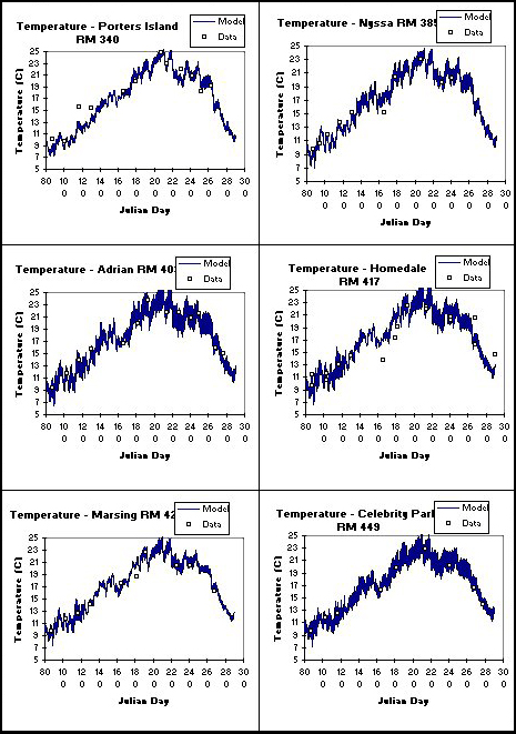
Figure 20. Computed versus observed temperatures in the Lower Snake River.
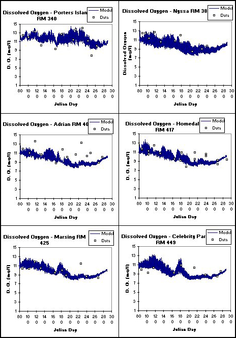
Figure 21. Computed versus observed dissolved oxygen in the Lower Snake River.
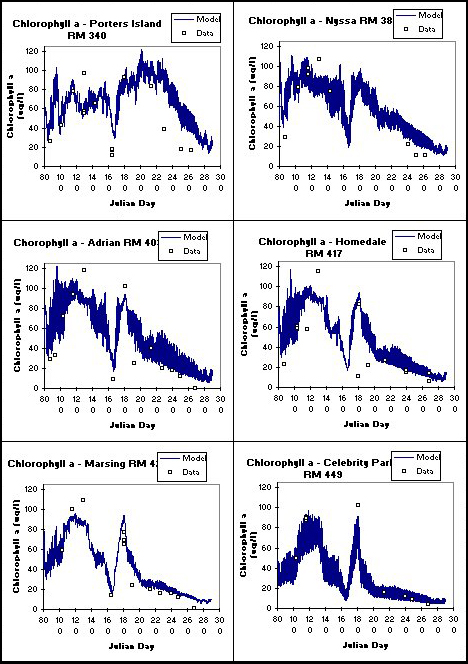
Figure 22. Computed versus observed chlorophylla.
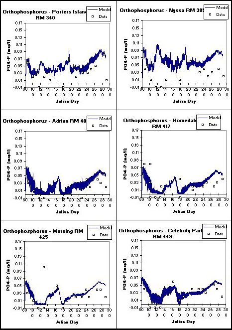
Figure 23. Computed versus observed dissolved PO4-P in the Lower Snake River.
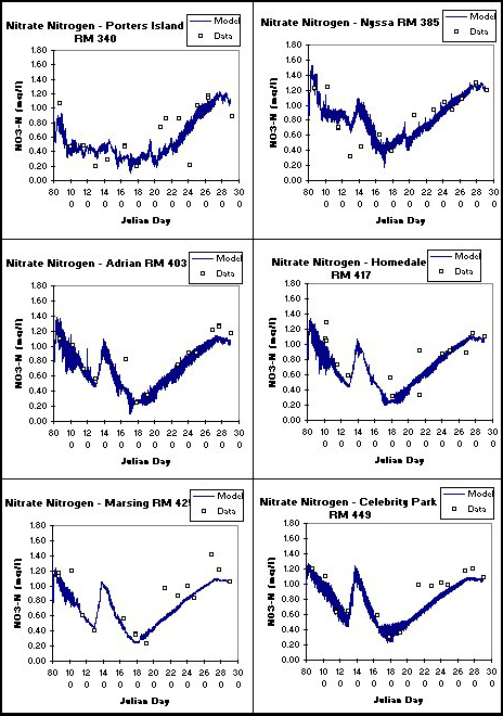
Figure 24. Computed versus observed nitrate/nitrite.
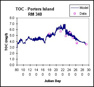
Figure 25. Computed versus observed total organic carbon (TOC).
Bull Run River System
The Bull Run watershed has been the primary drinking water supply since 1895 for the metropolitan area of Portland, OR, USA. The watershed is composed of two man-made reservoirs (Reservoir 1 and 2), and a potential third reservoir. Because of compliance requirements for endangered species survival, the reservoirs and river segments in the watershed were modeled with Version 3 in order to meet temperature standards for fish. Figure 26 shows the profile of the model system including two river and three reservoir sections. River channel slope was, on average, greater than 2% in the Upper Bull Run River.
A dye study performed in the Lower Bull Run River during June 1999 was used as a basis to verify the river model travel times and dispersive characteristics. Model-data comparisons are shown in Figure 27 using the Quickest-Ultimate numerical scheme.
Model predictions of temperature profiles in the two reservoirs during a two-year continuous simulation period were within 0.5oC Absolute Mean Error and 0.6oC Root Mean Square error for over 40 profile comparisons in each reservoir. A typical series of model-data predictions for Reservoir 1 are shown in Figures 28 and 29. Note how the model captures the double thermocline in late summer for Reservoir 1 and the differences between the thermal regimes in the two reservoirs. All hydrodynamic/temperature coefficients were set to their default values except for wind-sheltering.
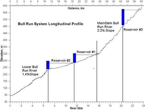
Figure 26. Bull Run River-Reservoir system profile.
Figure 27. A comparison of computed versus observed dye concentrations in the Lower Bull Run River during June 1999.
Figure 28. Model-data temperature profile comparisons for Reservoir 1 during 1997.

Figure 29. Model-data temperature profile comparisons for Reservoir 2 during 1997.
Columbia Slough System
The Columbia Slough (figure 30) is an extensive system of interconnected wetlands, channels, and lakes located in the Portland, Oregon, USA metropolitan area and lying in the floodplain of the Columbia River. It is approximately 30 km in length and includes a fresh-water estuary portion and a series of isolated lakes and channels that receive stormwater and groundwater inflows. The model was developed to evaluate the effect of combined sewer overflows, stormwater, and groundwater inflows on water quality in the Columbia Slough system. The model development is summarized in Berger and Wells [9].
The Lower Columbia Slough (Figure 31), is connected to the Willamette River where it experiences a tidal fluctuation of its water surface of between 1 to 3 ft. Inflows to the Lower Columbia Slough include combined-sewer-overflows (CSOs), storm water, water from Smith and Bybee Lakes, leachate from the St. John's Landfill, and inflows (both pumped and gravity inflows) from the Upper Columbia Slough at MCDD1.
The Upper Columbia Slough, shown in Figure 32, was historically maintained to provide irrigation water to agricultural and commercial users in the summer months. The Upper Slough is connected by pipes and an overflow weir during the Fall, Winter, and Spring to Fairview Lake. During the summer, Fairview Lake is connected to the Upper Slough only by flow over and leakage through the weir. Water is also pumped from the Upper Slough to the Lower Columbia Slough at a pump station at MCDD1 (Multnomah County Drainage District #1) and from the Upper Slough to the Columbia River at MCDD4(Multnomah County Drainage District #4). At MCDD1, pipes also allow gravity flow from the Upper Slough to the Lower Slough. Other inflows to the Upper Columbia Slough include groundwater and storm water from the Portland International Airport and other industrial, commercial, and residential neighborhoods in the area.
Figure 30. Columbia Slough.
Figure 31. Lower Columbia Slough.
Figure 32. Upper Columbia Slough.
The model’s ability to reproduce velocities in the tidally dominated Lower Slough is shown in Figure 33 during high-water conditions. CE-QUAL-W2 velocity predictions are laterally averaged whereas velocity measurements were taken at the channel center.
Figure 33. Measured centerline vertical velocity profiles compared to laterally averaged model predictions
during high-water conditions in the Lower Slough.
The model’s ability to reproduce water surface elevations in the Upper Slough is shown in figure 34. Note that the model is capable of reproducing the effects of water hammer on the water surface due to pumping operations.
Figure 34. Computed versus observed water surface elevations for Columbia Slough.
Figure 35. Computed versus observed flows for the Upper Slough.
Summary
A 2-D hydrodynamic and water quality model, CE-QUAL-W2 Version 3, has been developed for river basin modeling that allows the integration of river, reservoir, lake, and estuarine systems. Four test cases were shown demonstrating the ability of the model to reproduce river and tidal hydraulics and temperature and DO dynamics in stratified reservoirs.
References
-
[1] Cole, T. and Buchak, E. "CE-QUAL-W2: A Two-Dimensional, Laterally Averaged, Hydrodynamic and Water Quality Model, Version 2.0," Tech. Rpt. EL-95-May 1995, Waterways Experiments Station, Vicksburg, MS, 1995.
-
[2] Smith, D.J. "WQRRS, Generalized computer program for River-Reservoir systems," USACE Hydrol.Engr. Center, Davis, CA, 1978.
-
[3] Corps of Engineers. "HEC-5 Simulation of Flood Control and Conservation Systems," CPD-5Q, Hydrologic Engineering Center, Davis, CA, 1986.
-
[4] Donigian, A.S., Jr., J.C. Imhoff, B.R. Bicknell and J.L. Kittle, Jr. "Application Guide for Hydrological Simulation Program Fortran (HSPF)," EPA-600/3-84-065, U.S. Envir. Prot. Agency, Athens, GA, 1984.
-
[5] Ambrose, R. B.; Wool, T.; Connolly, J. P.; and Schanz, R. W. "WASP4, A Hydrodynamic and Water Quality Model: Model Theory, User's Manual, and Programmer's Guide," Envir. Res. Lab., EPA 600/3-87/039, Athens, GA, 1988.
-
[6] Environmental Laboratory "CE-QUAL-RIV1: A Dynamic, One-Dimensional (Longitudinal) Water Quality Model for Streams: User's Manual," Instr. Rpt. EL-95-2, USACE Waterways Experiments Station, Vicksburg, MS, 1995.
-
[7] Wells, S. A. "River Basin Modeling Using CE-QUAL-W2 Version 3," Proc . ASCE Inter.Water Res. Engr. Conf., Seattle, WA, 1999.
-
[8] Wells, S. A. "Theoretical Basis for the CE-QUAL-W2 River Basin Model," Dept. of Civil Engr., Tech. Rpt. EWR-6-97, Portland St. Univ., Portland, OR, 1997.
-
[9] Berger, C. and Wells, S. "Hydraulic and Water Quality Modeling of the Columbia Slough, Volume 1: Model Description, Geometry, and Forcing Functions," Dept. of Civil Engr., Tech. Rpt. EWR-2-99, Port. St. Univ., Portland, OR, 1999.